Authors:
(1) Xiaofan Yu, University of California San Diego, La Jolla, California, USA ([email protected]);
(2) Anthony Thomas, University of California San Diego, La Jolla, California, USA ([email protected]);
(3) Ivannia Gomez Moreno, CETYS University, Campus Tijuana, Tijuana, Mexico ([email protected]);
(4) Louis Gutierrez, University of California San Diego, La Jolla, California, USA ([email protected]);
(5) Tajana Šimunić Rosing, University of California San Diego, La Jolla, USA ([email protected]).
Table of Links
8 Evaluation of LifeHD semi and LifeHDa
9 Discussions and Future Works
10 Conclusion, Acknowledgments, and References
5 LIFEHD
In this section, we present the design of LifeHD, the first unsupervised HDC framework for lifelong learning in general edge IoT applications. Compared to operating in the original data space, HDC improves pattern separability through sparsity and high dimensionality, making it more resilient against catastrophic forgetting [52]. LifeHD preserves the advantages of HDC in computational efficiency and lifelong learning, while handling the input of unlabeled streaming data, which has not been achieved in previous work [18, 21, 22, 41, 65].
5.1 LifeHD Overview
Fig. 4 gives an overview of how LifeHD works. The first step is HDC encoding of data into hypervectors as described in Sec. 3. Training samples 𝑋 are organized into batches of size 𝑏𝑆𝑖𝑧𝑒 and input into an optional fixed NN for feature extraction (e.g. for images and sound) and the encoding module. The encoded hypervectors 𝜙 (𝑋) are input to LifeHD’s two-tier memory design inspired by cognitive science studies [5], consisting of working memory and long-term memory. This memory system intelligently and dynamically manages historical patterns, stored as hypervectors and referred to as cluster HVs. As shown in Fig. 4, the working memory is designed with three components: novelty detection, cluster HV update and cluster HV merge. 𝜙 (𝑋) is first input into novelty detection step (1). An insertion to the cluster HVs is made if a novelty flag is raised, otherwise 𝜙 (𝑋) updates the existing cluster HVs (2). The third component, cluster HV merge (3), retrieves the cluster HVs from long-term memory, and merges similar cluster HVs into a supercluster via a novel spectral clustering-based merging algorithm [59]. The interaction between working and long-term memory happens as commonly encountered cluster HVs are copied to long-term memory, which we call consolidation (4). Finally, when the size


limit of either working or long-term memory is reached, the least recently used cluster HVs are forgotten (5).
ecently used cluster HVs are forgotten (○5 ). All modules in LifeHD work collaboratively, making it adaptive and robust to continuously changing streams without relying on any form of prior knowledge. For example, in scenarios of distribution drift, LifeHD may generate new cluster HVs upon encountering drifted samples initially, which can later be merged into coarse clusters. This approach ensures that LifeHD can efficiently capture and retain historical patterns.
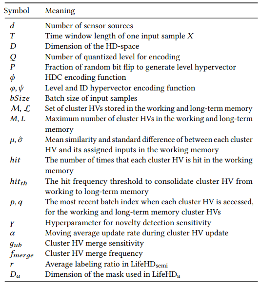
In the following, we discuss more details about the major components of LifeHD: novelty detection (Sec. 5.2), cluster HV update (Sec. 5.3), and cluster HV merging (Sec. 5.4). We summarize the important notations used in this paper in Table 1.
5.2 Novelty Detection
The initial novelty detection step (1 in Fig. 4) is crucial for identifying emerging patterns in the environment. SupposeM = {𝑚1, ...,𝑚𝑀} is the set of cluster HVs stored in the working memory. We gauge the "radius" of each cluster by tracking two scalars for each cluster HV 𝑖: 𝜇𝑖 and 𝜎ˆ𝑖 , which represent the mean cosine difference and standard difference between the cluster HV and its assigned inputs. Given 𝜙 (𝑋), we first identify the most similar cluster HV, denoted by 𝑗. LifeHD marks 𝜙 (𝑋) as “novel" if it substantially differs from its nearest cluster HV. Specifically, this dissimilarity is measured by comparing cos(𝜙 (𝑋),𝑚𝑗) with a threshold based on the historical distance distribution of cluster HV 𝑗:

The hyperparameter 𝛾 fine-tunes the sensitivity to novelties.
LifeHD recognizes new 𝜙 (𝑋) as prototypes and inserts them into the working memory. When reaching its size limit 𝑀, the working memory experiences forgetting (○5 in Fig. 4). The least recently used (LRU) cluster HV, represented by 𝐿𝑅𝑈 = argmin𝑀 𝑖=1 𝑝𝑖 , is replaced. Here 𝑝 corresponds to the latest batch index where the cluster HV was accessed. A similar forgetting mechanism is configured for the long-term memory, where the last batch accessed is marked with 𝑞.
5.3 Cluster HV Update
If novelty is not detected, indicating that 𝜙 (𝑋) closely matches cluster HV 𝑗, we proceed to update the cluster HV and its associated information (2 in Fig. 4). This update process involves bundling 𝜙 (𝑋) with cluster HV 𝑚𝑗 , akin to how class hypervectors are updated as described in Sec. 3, and updated 𝜇𝑗 and 𝜎ˆ𝑗 with their moving average

The hyperparameter 𝛼 adjusts the balance between historical and recent inputs, where a higher 𝛼 gives more weight to recent samples. Properly maintaining 𝜇𝑗 and 𝜎ˆ𝑗 is vital for tracking the “radius” of each cluster HV, affecting future novelty detection. We also increase the hit frequency ℎ𝑖𝑡𝑗 and refresh 𝑝𝑗 with current batch index 𝑖𝑑𝑥. ℎ𝑖𝑡𝑗 is further used to compared with a predetermined threshold ℎ𝑖𝑡𝑡ℎ to decide when a working memory cluster HV appears sufficiently frequently to be consolidated to long-term memory (4 in Fig. 4). 𝑝𝑗 determines forgetting as described in the previous section. With this lightweight approach, LifeHD continually records temporal cluster HVs from the environment, while the most prominent cluster HVs are transferred to long-term memory.

5.4 Cluster HV Merging
Cluster HV merge (3 in Fig. 4) has the dual benefit of reducing memory use and of elucidating underlying similarity structure in the data. Intuitively, a group of cluster HVs can be merged if they are similar to each other and dissimilar from other cluster HVs. For instance, one might merge the cluster HVs for Bulldog and Chihuahua into a single “Dog” cluster HV, that remains distinct from the cluster HV for “Tabby Cat”.
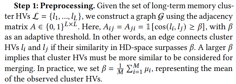
To merge the cluster HVs, we first construct a similarity graph defined over the cluster HVs from the long-term memory. The cluster HVs correspond to nodes, and a pair of cluster HVs are connected by an edge if they are sufficiently similar. We then merge the cluster HVs by computing a particular type of cut in the graph in a manner similar to spectral clustering [40]. This graph based formalism for clustering is able to capture complex types of cluster geometry and often substantially outperforms simpler approaches like K-Means [59]. We detail the steps of cluster HV merging in LifeHD below, while Fig. 5 offers an illustrative overview.

Step 2: Decomposition. We compute the Laplacian𝑊 = 𝐷 −𝐴, where 𝐷 is the diagonal matrix in which 𝐷𝑖𝑖 = Í 𝑗 𝐴𝑖𝑗 . We then compute the eigenvalues 𝜆1, .., 𝜆𝐿, sorted in increasing order, and eigenvectors 𝜈1, ..., 𝜈𝐿 of 𝑊.
Step 3: Grouping. We infer 𝑘 = max𝑖∈ [𝐿] 𝜆𝑖 ≤ 𝑔𝑢𝑏, and merge the cluster HVs by running K-Means on 𝜈1, ..., 𝜈𝑘 . The upperbound 𝑔𝑢𝑏 is a hyperparameter that adjusts the granularity of merging, with a smaller 𝑔𝑢𝑏 leading to smaller 𝑘 thus encouraging merging more aggressively.
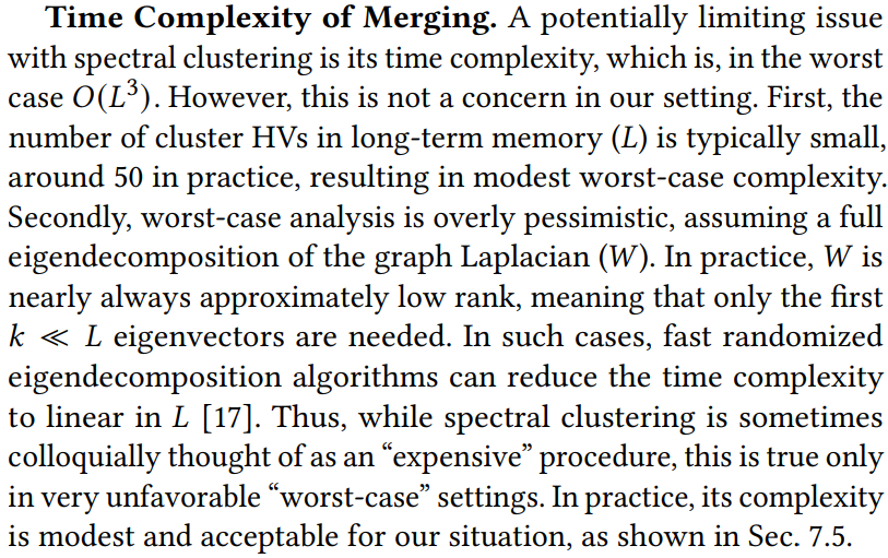
Our merging approach is formally grounded, as discussed in [59]. It is a well-known fact that the eigenvectors of 𝑊 encode information about the connected components of G. When G has 𝑘 connected components, the eigenvalues 𝜆1 = 𝜆2 = ... = 𝜆𝑘 = 0. To recover these components, K-Means clustering on 𝜈1, ..., 𝜈𝑘 can be employed, as explained in [59]. However, practical scenarios may have a few inter-component edges that should ideally be distinct. For instance, when the similarity threshold is imprecisely set, erroneous edges may appear in the graph, causing 𝜆1, ..., 𝜆𝑘 to be only approximately zero. Our merging approach is designed to handle this situation by introducing 𝑔𝑢𝑏. The cluster HV merging is evaluated every 𝑓𝑚𝑒𝑟𝑔𝑒 batches, where 𝑓𝑚𝑒𝑟𝑔𝑒 is a hyperparameter that controls the trade-off between merging performance and computational latency. Both 𝑔𝑢𝑏 and 𝑓𝑚𝑒𝑟𝑔𝑒 are analyzed in Sec. 7.8, along with other key hyperparameters in LifeHD.

This paper is available on arxiv under CC BY-NC-SA 4.0 DEED license.

